TUTORIAL 2: Tutorial on how to get AVERAGE and to use vlookup in OpenOffice Calc

Let’s say, you are a Chemistry teacher, and in your class, you had four (4) Term Examinations. Your student, Eldridge, got the following scores: 64/100, 62/100, 58,100 and 59/100. If the passing score is 60, which is equivalent to 3.00; what will be your student’s average and his corresponding final grade? Will he pass the subject?

Well, in this tutorial, I am going to show you how to compute the average and to indicate the equivalent or corresponding grades of your students using vlook-up in OpenOffice Calc. The version of OpenOffice used in this tutorial is Apache OpenOffice 4.1.1.

Below is an example of a data sheet containing student’s names and their corresponding grades in a particular examination. 
Note: All of the students names and scores which appeared herewith are only  hypothetical and do not reflect their real performance in class. This is for description and visual purposes only.  

   To compute for the AVERAGE:

Step 1: Click on the cell to parallel to the student’s names and term exams grades, enter equal ( = ) sign; type AVERAGE()

 Step 2: Drag the cells that you are determining the average; that is, the student's term examinations grades. 

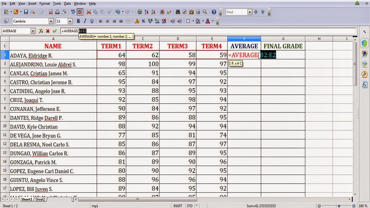
Step 3: Press ENTER. You now have the student's AVERAGE in all his four term examinations! 

Now, in order for you to get all your student's average, you don't need to do the same procedures repeatedly! Instead, you can just drag the same formula until the end of your data sheet. 

Step 4: When you point the pointer at lower right corner of the cell where you had just computed the average, a plus (+) sign will appear. Click it and drag it (by holding it without releasing) until you reach the last cell of your data sheet, and then release. 

You now have the average scores of the students in your class! Your next target is, to determine the FINAL GRADE of your students. 

It is unnecessary for you to type individually the final grade of your students. We now have the role of vlook-up to answer this! 

But before you can compute for the final grade, you need to have a look-up table. It is where the average scores will have its equivalent grades. In order to do this, you must have another data sheet (Sheet 2) that is separate from your original data sheet (Sheet 1).

Step 1: Make and edit your table accordingly. Be sure you are doing this on another data sheet! 

Since we already have our look-up table, where each average scores has its equivalent grade, the final grade can be now computed. 

To compute for the FINAL GRADE:

Step 1: Click on the cell to parallel to the student’s average, enter equal ( = ) sign; type VLOOKUP(

Step 2: Click on the Function sign(fx) on top left of the table. Another tab will show up (Function Wizard).

Step 3: The Search_criterion is the Average. For the array, it is the Look-up table (Sheet 2). For the Index, just type number 2. Lastly, for the sort_order, type TRUE. 
     Step 3.1: Search criterion: AVERAGE

     Step 3.2: Array: Look-up table on Sheet 2

   Step 3.3: Index: type 2; sort_order: type TRUE.

Step 4: Click on OK. You now have the final grade of that student, Eldrige, which is 3. This means he PASSED Chemistry!

Now, in order for you to get all your student's final grades, you don't need to do the same procedures repeatedly!  Instead, you can just drag the same formula until the end of your data sheet. 

Step 5: When you point the pointer at lower right corner of the cell where you had just computed the average, a plus (+) sign will appear. Click it and drag it (by holding it without releasing) until you reach the last cell of your data sheet, and then release. 

Congratulations! You now have the average and the final grades of the students! 

Want to know how many of your students got 3.00? ? Or how many got 1.00 and so on? 

We can compute this by using Count-If. 

It is important that we place this statistics of grades on separate sheet, aside from your original sheet (Sheet 1). 

To compute for the statistics of the grades:

Step 1: Click on the cell parallel to the grade. Type the equal sign ( = ), and type COUNTIF(

Step 2: Click the Function sign (fx) on top left of the table. Another tab (Function Wizard) will appear, which asks you the Range and Criteria. 

Step 3: The Range is the Final Grade on Sheet 1, and the Criteria is the Grade on Sheet 2. For the range, just drag the whole Final grade up to the last cell of the data, and do the same for the grade. 

      Step 3.1: Select Range

Step 3.2: Select Criteria

Step 3.3: Another tab will appear showing the range and criteria you have selected. Click OK.

Step 4: By clicking OK, you will now have the number (count) of students having a grade of 3. Just drag down to get the counts for the remaining grades. 

Step 5: Make sure you got the same total number of students. To check, enter another cell just below your last count. Type equal sign ( = ), type SUM(, then drag the whole cells under count. 

If you want to know the corresponding percentage of a particular grade, then: 

  Step 6: Type equal sign ( = ), then click the cell under count, the division sign ( / ), then click the total count. To have the absolute value, just type a dollar sign($) in between the name of the total count. Hit Enter. 

Step 7: Press Enter.

Step 8: Just drag down until you reach the last cell of your data to get the percentage of the whole data. Make sure you'll get 100%. 

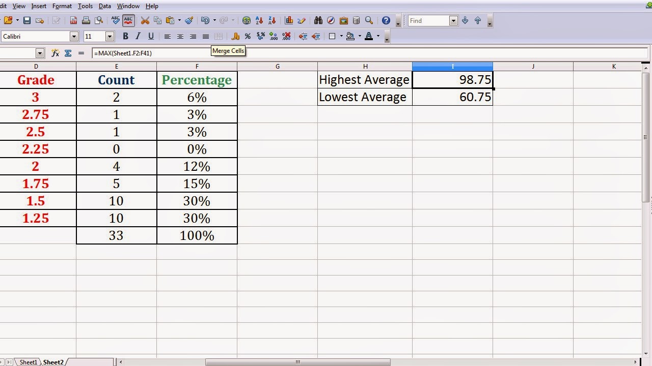
If you want to know the highest and lowest grades of your students:

Step 9: In getting the highest average, type equal sign ( = ), then type MAX(

Step 10: Highlight the whole Average in Sheet 1. 

Step 11: By pressing ENTER, you'll be getting the highest grade of your students.

To get the lowest grade of your students:

Step 12: Type equal sign ( = ), type MIN(

Step 13: Highlight the whole Average on Sheet 1.

Step 14: By pressing ENTER,  you'll be getting the lowest grade of your students.

Good thing, all of your students passed your subject, Chemistry! :)

Thank you! 

Please read my other tutorials! :)

All Rights Reserved (2014)
Intellectual Property of:
Josephine Joy V. Tolentino
Master of Science in Biology student
College of Arts and Sciences
Department of Biological Sciences
Central Luzon State University
Science City of Munoz, Nueva Ecija
   Philippines